| |
|
|||||||
|
|
||||||||
|
Simulator InterconnectionWe describe a laboratory experiment that addresses decentralized control, where the individual controllers are connected by a digital communication network. In the particular experiment, there are two controller components and one plant component, each simulated by an instance of the simulator simfaudes, executed on a dedicated PC. The purpose of the example is to demonstrate how the three simulations use specific I/O devices in order to synchronize their respective events. Variations of this example have been used to test an implementation of the D3RIP realtime network protocols. 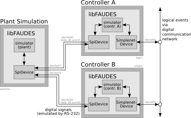
LRT laboratory setup: decentralized control and plant simulation on 3 PCs Configuration files and related scripts can be found in the tutorial directory of the iodevice plug-in and are prefixed decdemo_*. Plant SimulationThe plant under consideration is a variant of the common simple machine scenario, however, modelled as a physical system with digital I/O signals as given in the below table. The bit address (last column) is used to identify individual signals and may refer to an actual wiring and the corresponding configuration of a libFAUDES SignalDevice. In the particular laboratory setup, we use emulated digital signals via serial interfaces, as provided by the SpiDevice. There, bit addresses refer to the layout of the so called process image.
The signals P_ACTUATOR and M_ACTUATOR are plant inputs, i.e. line levels can be set by a controller at any time to any value. The signals P_SENSOR and M_SENSOR are plant outputs, i.e. line levels will be set by the plant according to its respective state. The below figures indicate the respective signals for normal operation (left) and machine break-down with subsequent maintenance (right). 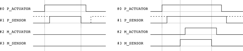
LRT laboratory setup: signals for intended operation (left) and break-down-maintenance cycle (right). Technical detail. We will use controllers that ignore positve edges on P_SENSOR. Thus, it does not matter at which time the positive edge occurs, as long as on completion of the process the line level is high to allow for a negative edge. The plant dynamics are modelled in terms of events that correspond to edges on the input- and output-signals; see also SignalDevice and/or the elevator example. Note that the plant model will allow for any actuator events at any time and it will be the task of the two controllers to achieve the intendend behaviour.
An according configuration of an SpiDevice is provided by the file decdemo_plant_serial.dev: % Device configuration for serial process image device <SpiDevice name="plant simulator"> <!-- Time scale in ms/ftu --> <TimeScale value="1000"/> <!-- Sample interval for edge detection in us (10ms) --> <SampleInterval value="10000"/> <!-- Role: master --> <Role value="master"/> <!-- Sytem device files --> <DeviceFile value="/dev/ttyS1"/> <DeviceFile value="/dev/ttyS2"/> <!-- Event definitions --> <EventConfiguration> <Event name="p_start" iotype="input"> <Triggers> <PositiveEdge address="0"/> </Triggers> </Event> <Event name="p_stop" iotype="input"> <Triggers> <NegativeEdge address="0"/> </Triggers> </Event> <Event name="p_inprog" iotype="output"> <Actions> <Set address="1"/> </Actions> </Event> <Event name="p_complete" iotype="output"> <Actions> <Clr address="1"/> </Actions> </Event> <Event name="m_start" iotype="input"> <Triggers> <PositiveEdge address="2"/> </Triggers> </Event> <Event name="m_stop" iotype="input"> <Triggers> <NegativeEdge address="2"/> </Triggers> </Event> <Event name="m_request" iotype="output"> <Actions> <Set address="3"/> </Actions> </Event> <Event name="m_complete" iotype="output"> <Actions> <Clr address="3"/> </Actions> </Event> </EventConfiguration> </SpiDevice> With respect to the above events, the plant dynamics are modelled by the synchronous product of the below generators:
In order to obtain realistic behaviour w.r.t. timing, we use stochastic execution attributes for the events p_complete, m_request and m_complete as specified by the below simfaudes configuration file; see also the ProposingExecutor. Effectively, the parameters amount to a stochastic process duration with a mean of 75ftu and stochastic machine break-down with a mean of 200ftu processing time. % Configuration for plant simulator <Executor> % Specify generators <Generators> "decdemo_planta.gen" "decdemo_plantb.gen" </Generators> % Specify event attributes <SimEventAttributes> % Dont propose inpute events "p_start" <Priority> -50 </Priority> "p_stop" <Priority> -50 </Priority> "m_start" <Priority> -50 </Priority> "m_stop" <Priority> -50 </Priority> % Timing "p_inprog" <Priority> 50 </Priority> "p_complete" <Stochastic> +Trigger+ +Gauss+ <Parameter> 50 100 75 20 </Parameter> </Stochastic> "m_complete" <Stochastic> +Trigger+ +Gauss+ <Parameter> 50 100 75 20 </Parameter> </Stochastic> "m_request" <Stochastic> +Delay+ +Gauss+ <Parameter> 150 250 200 20 </Parameter> </Stochastic> </SimEventAttributes> </Executor> For an interactive simulation of the plant, open a command shell and change to the iodevice tutorial directory to run simfaudes $ cd ./libfaudes/plugins/iodevice/tutorial $ ../../../bin/simfaudes -v -i data/decdemo_plant.sim Controller ConfigurationThere are two designated controllers in our setup. Controller A runs the plant by the signals P_ACTUATOR and P_SENSOR and is meant to schedule the processing of workpieces as long as there is no maintenance required. Controller B is connected by the signals M_ACTUATOR and M_SENSOR and is meant to controll the maintenance cycle after break-down. The below tables define the events for the respective controller in one-to-one correspondance with the plant model. Note, however, that plant inputs become controller outputs and vice versa.
The respective configuration of SpiDevices is provided by the files decdemo_contra_serial.dev and decdemo_contrb_serial.dev. We give a listing for Controller A: %Device configuration for serial process image device <SpiDevice name="ControllerA_Serial"> <!-- Time scale in ms/ftu --> <TimeScale value="10"/> <!-- Sample interval for edge detection in us (1ms) --> <SampleInterval value="1000"/> <!-- Role: slave --> <Role value="slave"/> <!-- Sytem device file --> <DeviceFile value="/dev/ttyS0"/> <!-- Events --> <EventConfiguration> <Event name="p_start" iotype="output"> <Actions> <Set address="0"/> </Actions> </Event> <Event name="p_stop" iotype="output"> <Actions> <Clr address="0"/> </Actions> </Event> <Event name="p_inprog" iotype="input"> <Triggers> <PositiveEdge address="1"/> </Triggers> </Event> <Event name="p_complete" iotype="input"> <Triggers> <NegativeEdge address="1"/> </Triggers> </Event> </EventConfiguration> </SpiDevice> Our intention is to mimique the behaviour of the common simple machine example, stated in terms of the abstract events alpha (start process), beta (process completed), mue (break-down), and, lambda (maintenance completed). The below controllers are meant to control the plant and to schedule the abstract events in compliance with the intended semantics.
The designated closed-loop behaviour amounts to K := Ga||Gb||Ca||Cb, and, indeed, the projection to the high level alphabet {alpha, beta, mue, lambda} resembles the common simple machine. The tutorial directory provides the Lua script decdemo_verify.lua that verifies that relevant controllability conditions are satisfied, i.e., that in the closed-loop configuration neither controller disables sensor events and that the plant never disables actuator events. This is not surprising, since we've based our modells on physical input-output signals.
Each controller only refers to those plant events, that it can access via the direct interconnection by input-signals and output-signals. However, both controllers share the abstract event lambda which must be synchronized in order to obtain the closed-loop behaviour K. It is verified in decdemo_verify.lua that K is controllable w.r.t. Cb and the uncontrollable events {m_start, m_stop, lambda}. Thus, the event lambda is never disabled by K when it is enabled in Cb. For the particular example, it can also be seen that whenever lambda is enabled in Controller B, the other controller cannot execute any other event, i.e., Controller A waits for lambda. Hence, the execution of lambda can be decided locally by Controller B, which is meant to indicate any such execution to Controller A. In the laboratory experiment, we use a SimplenetDevice to communicate the execution of lambda over a TCP/IP network, configured as follows:
The overall device configuration is given by the files decdemo_contra.dev and decdemo_contrb.dev, which gather the respective serial- and network devices as a container device; see also DeviceContainer. Simulation parameters are specifed in decdemo_contra.sim and decdemo_contrb.sim, respectively. They amount to a short delay befor starting a process by alpha to ensure edge detection. Closed-Loop SimulationHardware configuration and testing.Assuming that all three PCs are running a similar Linux distribution and are accessible via a network, it is most convenient to use one machine for compilation/configuration and to distribute the relevant files to the other PCs by a shell script. An example is provided in decdemo_upload.sh, which should be easy to adapt for other hostnames/logins etc. For the serial interfaces, two null-modem cables are required to connect the three PCs as indicated by the figure at the top of this page. The current implementation of the SpiDevice does no hardware handshake, so three-wire cables will be fine (using TxD, RxD and Gnd). One may use any terminal program to figure the respective system device files, (typically /dev/ttySnn or /dev/ttyUSBnn for USB-to-serial adapters), and to test the serial interconnection. We found cutecom particulary useful for that purpose. Once the device files are known, the configuration files decdemo_plant_serial.dev, decdemo_contra_serial.dev, and decdemo_contrb_serial.dev need to be adapted accordingly. It is recommended to test the overall configuration by running the iomonitor (provided by libFAUDES in the bin directory) on each PC. plant_simulator_pc$ ./iomonitor decdemo_plant_serial.dev controller_a_pc$ ./iomonitor decdemo_contra.dev controller_b_pc$ ./iomonitor decdemo_contrb.dev With the iomonitor, execute any output event from any PC via the we command and check for the event to be delivered to the remaining PCs by rf. Starting the simulation.The recommended order is to first start the plant, then Controller B, and finally controller A. plant_simulator_pc$ ./simfaudes -v -d decdemo_plant_serial.dev decdemo_plant.sim controller_b_pc$ ./simfaudes -v -d decdemo_contrb.dev decdemo_contrb.sim controller_a_pc$ ./simfaudes -v -d decdemo_contra.dev decdemo_contra.sim libFAUDES 2.34g --- 2026.04.28 --- with "omegaaut-synthesis-observer-observability-diagnosis-hiosys-iosystem-multitasking-coordinationcontrol-timed-simulator-iodevice-priorities-luabindings-hybrid-example-pybindings" |
||||||||||||||||||||||||||||||||||||||||||||||||||||||||||||||||||||||||||||||||||||||||||||||||||||||||||||||||||||||||||||||||||||


