| |
|
|||||
|
|
||||||
Manufacturing System Simulator
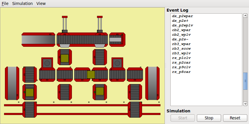
The plant simulator FlexFact mimics the dynamical behaviour of various electro-mechanical components, like conveyor belts and processing machines, to form a flexible manufacturing system. FlexFact is easily configurable, i.e. the user can choose and place components in order to design their very own factory layout.
FlexFact components are a superset of those used for the LRT production line laboratory model, available for puchase at Staudinger GmbH. Regarding the interconnection with a controller, either implemented by a PLC or natively by libFAUDES, a FlexFact simulation is meant to behave like the respective physical system.
General Note on using FlexFact. The simulator is intentionally implemented as a completely self-contained executable, readily installed to play along. However, as with a physical plant, you will need some controller to run the simulator according to your specifications and you must effectively configure all wiring between plant and controller to form a closed loop. FlexFact provides some assistance for the wiring, however, the overall effort required to set up the closed loop must not be under-estimated. In this regard, the simulation is quite realistic.
Plant Configuration
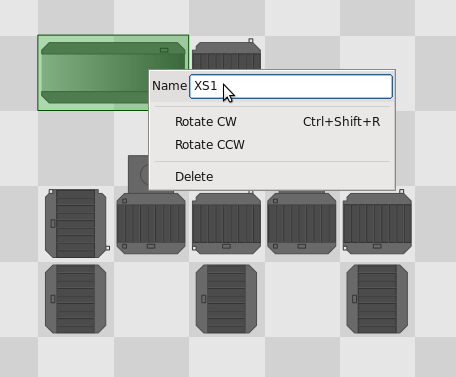
On start-up, FlexFact shows an empty factory floor. Plant components can be added by the context menu, i.e. right-click on the position where you would like to place a component and select the component type from the pop-up menu. Be sure, that the position to insert is not allocated by some other component from you factory.
Every component is identified by a unique name. The default consists of a two-letter-abbreviation of the component type and a numeric value to distinguish multiple components of the same type; e.g. CB1, CB2, CB3 for three conveyor belts. You can re-name components by their context-menu.
Components can be selected and moved around by mouse click and drag, respectively. To rotate or further configure parameters of a component, again use their context menu.
The plant configuration can be saved to or loaded from file via the File menu. The file extension defaults to *.ffs. Examples are provided in the examples folder.
Simulation
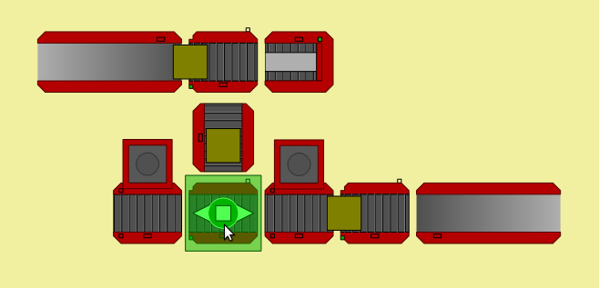
The start/stop/reset buttons on the bottom right of the FlexFact window control the simulation. When starting the simulation, nothing seems to happen. This is because all actuators initially are passive. However, while running the simulation without any controller connected, the individual components context menu allows to change input line-levels, e.g. to turn on the motor of a conveyor belt. Most components also offer some sensible manual operation, e.g. turn rotary table to the other orientation, or feed a workpiece. Thus, you can operate the factory manually to inspect particular aspects of it's behaviour.
The simulator should be fine, as long as each component is operated in the intended way. Transport of workpieces is treated as if it was implemented by "magnetic rails". Thus, minor positioning errors due to timing issues will be annihilated. Similarly, the rotary tables will snap into their intended position "magnetically". However, when the simulator recognises a situation that it can not handle properly, the respective workpieces are marked to be removed by mouse click. This is the case, e.g., when attempting to turn a rotary table with a workpiece only partly on the belt, or, when a workpiece drops from a conveyor belt. When completely stuck, the simulation must be reset.
External Interface
Interaction with a controller is motivated physically and implemented by virtual external signals. At any instance of time, each signal takes one of the two boolean values "true" or "false". Actuator signals are inputs to the simulator and e.g. determine whether or not a motor is running. Sensor signals are outputs from the simulator and indicate e.g. whether a key-switch is activated or not. The boolean vector of all signals (arranged in alphabetical order) is referred to as the process image.
You can inspect the process image on the right column of the simulator window; see also the View menu. Individual signals are identified by their symbolic name, which is upper-case and of the form XXXX_YYYY, where XXXX is the component name and YYYY identifies the signal relative to the component. E.g. CB1_BM+ is the input signal to control the belt motor of conveyor belt CB1. See the below documentation of the individual components for further details.
FlexFact provides two interfaces for a controller to access the process image. A Modbus/TCP Slave is implemented to directly access the process image via the Modbus protocol, and, there is a libFAUDES Simplenet device to communicate events defined as particular edges on specific signals from the process image. You can activate either interface via the Simulation Menu.
Modbus/TCP interface
For the Modbus/TCP interface, the simulator takes the server role and listens at TCP port 1502 for a client to connect. It is up to the client which output values to request and which input values to set. The pragmatic approach for a PLC program is to maintain a local copy of the process image and to update it once per cycle.
Address mapping is exactly as shown in the visual representation of the process image. Some PLCs introduce on offset of 1 in order to avoid a 0th line level. FlexFact implements bit-wise access, as well as register-wise access. The current version of FlexFact will silently ignore any attempt of the client to set a sensor line level. Thus, a PLC can read and write the entire image using Modbus multi-bit or multi-register access. FlexFact will issue address-out-of-range errors whenever a client request refers to a signal outside the actual process image.
Simplenet interface
With the libFAUDES Simplenet interface, not signal levels but discrete events form the basis of system interconnection. The latter are defined as edges on signals, either reported by FlexFact (sensor events) or imposed by the external peer (actuator events). Events are identified by their symbolic name, which is lower case and of the form xxxx_yyyy. Here, xxxx is the name of the respective component and yyyy identifies the event relative to the component. E.g. cb1_bm+ turns on the belt motor of the conveyor belt CB1 and cb1_wpar is indicates that a workpiece has arrived at the sensor of CB1. A detailed definition of the supported events is given below.
Note: Simplenet implements address resolution via UPD broadcasts (port 40000) to locate participating nodes anywhere in the entire subnet. For FlexFact, the Simplenet network name is derived from the factory setup filename. Thus, to run multiple instances of FlexFact within the same subnet, filenames must differ. Alternatively, you can choose Simplenet (local) from the Simulation menu for explicit address configuration restricted to the local machine. This is also a workaround when automatic address resolution fails.
Relevant libFAUDES tools
The libFAUDES command-line tool iomonitor comes with a Modbus client and a Simplenet implementation. Thus, the external interface can be tested and/or inspected by the iomonitor. The FlexFact File menu has an entry to generate the according libFAUDES device configuration.
To have a discrete event supervisor control the factory simulation, its dynamics must be imposed on FlexFact via the external interface. This can be done on various ways, most naturally by simulation of the supervisor with synchronized shared events using the the Simplenet interface. Here, the controller simulation may be done with the libFAUDES command-line tool simfaudes or with the DESTool built-in simulator. In both cases, the device configuration provided by FlexFact can be used to set-up the communication accordingly. For step-by-step instructions, see the the example "OperatorPanel" provided with the FlexFact package.
Note: For the current revision of the DESTool built-in simulator, we have experienced timing issues when controlling more than a view FlexFact components. In this regard, the libFAUDES command-line tool simfaudes is preferable. Here, the command-line option -qq reduces the latency to a couple of milliseconds.
Available Components
Find below a description of the components available for FlexFact simulations. To learn more about a particular component, it is instructive to set up a simple factory that utilises the component in question and to operate it manually (without an external interface).
Conventions
The below figures represent the respective component in default orientation and in initial state.
Directions (west, east, north and south) refer to the top-view on the factory and the default orientation of the component.
For west and north, we use the suffix -, while + indicates east or south (as in graphics coordinates for x- and y-axis).
Signal levels are defined such that the boolean value 0 (aka false or low) represents a passive state, e.g. motor off, no workpiece at sensor etc.
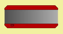
CB - Conveyor Belt
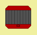
The conveyor belt is meant to transport workpieces. The motor is driven by two boolean signals, one for each direction. The two motor signals must not be active simultaneously.
In the middle of the belt, there is a sensor to detect workpieces. The sensor signal is active when a workpiece is present, i.e. if the center of the workpiece is within a defined range of the sensor.
The length of the conveyor belt can be configured, the example in the figure to the left is of length one. For longer conveyor belts, there are two workpiece sensors, one at west position and one at the east position.
| signals | description | events |
|---|---|---|
| CB_BM+, CB_BM- | motor, to the east or west, resp. | cb_bm+ (to the east), cb_bm- (to the west), cb_boff (stop) |
| CB_WPS | workpiece sensor | cb_wpar (positive edge, arrival), cb_wplv (negative edge, departure) |
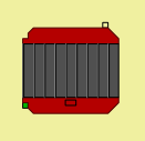
DS - Distribution System
The distribution system is a conveyor belt with a configurable number of perpendicular pushers. Typical usage is to take up workpieces on the belt and to distribute them to further components located south of the respective pusher.
Each pusher is equipped with a motor for movement in north-south direction and two key-switches that indicate arrival in the north-most or south-most position, respectively.
The conveyor belt is operated as the standard conveyor belt component, except that there is one workpiece sensor per pusher.
For the below definition of signals and events, we use Z to indicate the pusher number, starting with Z=1 for the west-most pusher and ranging up to the east-most pusher, i.e., Z=2 for the distribution system in the figure.
| signals | description | events |
|---|---|---|
| DS_BM+, DS_BM- | belt motor, to the east or west, resp. | ds_bm+ (to the east), ds_bm- (to the west), ds_boff (stop) |
| DS_PzWPS | workpiece sensor at pusher z | ds_pZwpar (positive edge, arrival), ds_pZwplv (negative edge, departure) |
| DS_PzM+, DS_PzM- | pusher Z motor, to the south or north, resp. | ds_pZm+ (to the south), ds_pZm- (to the north), ds_pZoff (stop) |
| DS_PzS+ | pusher Z south position | ds_pZs+ (positive edge, position reached) |
| DS_PzS- | pusher Z north position | ds_pZs- (positive edge, position reached) |
OP - Operator Panel
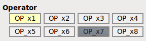
The operator panel provides a configurable number of push buttons and indicator lights for interaction of the controller with a human operator. While technically a plant component, the operator panel is shown together with the event log and the simulation controls. Configuration is via the Simulation Menu.
| signals | description | events |
|---|---|---|
| OP_Lz | indicator light no. z | op_lZon (positive edge), op_lZoff (negative edge) |
| OP_Sz | push button no. z | op_sZact (positive edge, button pressed), op_sZrel (negative edge, button released) |
PM - Processing Machine
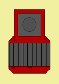
The processing machine can transport workpieces as the standard conveyor belt component. Once a workpiece has arrived at the sensor, the belt can be stopped for the machine to process the workpiece.
Processing is done in three stages. First, the machine is positioned above the workpiece, then, the actual process is performed, and finally, the machine is positioned back in its home position.
Machine positioning is done by a motor and two sensors, one for the home position (north) and one for the processing position (south). The actual process is enabled by the signal PM_MOP. A negative edge on PM_MRD indicates completion of the process.
| signals | description | events |
|---|---|---|
| PM_BM+, PM_BM- | belt motor, to the east or west, resp. | pm_bm+ (to the east), pm_bm- (to the west), pm_boff (stop) |
| PM_WPS | workpiece sensor | pm_wpar (positive edge, arrival), pm_wplv (negative edge, departure) |
| PM_PM+, PM_PM- | machine positioning motor, to the south or north, resp. | pm_pm+ (to the south, processing pos.), pm_pm- (to the north, home pos.), pm_poff (stop) |
| PM_PS+ | machine in south position | pm_ps+ (positive edge, processing pos. reached) |
| PM_PS- | machine in north position | pm_ps- (negative edge, home pos. reached) |
| PM_MOP | processing machine on | pm_mon (turn machine on), pm_moff (turn machine off) |
| PM_MRD | high, when ready to start processing machine on | pm_mrqu (positive edge, ready to start machine) pm_mack (negative edge, process completed) |
UM - Universal Machine
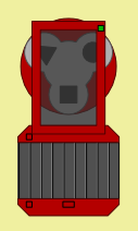
The universal machine can transport workpieces as the standard conveyor belt component and it can process a workpiece as the processing machine component. In addition, the univerversal machine can select one out of three tools to be applied during processing, i.e., the machine can be operated in three distinct processing modes.
Once a workpiece has arrived at the sensor, the belt can be stopped for the machine to process the workpiece. This is done in four stages. First, there is the option to select a processing tool. Second, the machine is positioned above the workpiece. Third, the actual process is performed, and finally, the machine is positioned back in its home position.
Tool selection is done by a motor that can be operated clockwise or counterclockwise, controlled by one signal each, and a sensor to indicate valid selections. Machine positioning is done by a motor and two sensors, one for the home position (north) and one for the processing position (south). The actual process is enabled by the signal UM_MOP. A negative edge on UM_MRD indicates completion of the process.
| signals | description | events |
|---|---|---|
| UM_BM+, UM_BM- | belt motor, to the east or west, resp. | um_bm+ (to the east), um_bm- (to the west), um_boff (stop) |
| UM_WPS | workpiece sensor | um_wpar (positive edge, arrival), um_wplv (negative edge, departure) |
| UM_TCW, UM_TCCW | tool selection motor, clockwise or counterclockwise, resp. | um_tcw (rotate clockwise), um_tccw (rotate counterclockwise), um_toff (stop) |
| UM_TS | tool selection sensor | um_trd (tool ready) |
| UM_PM+, UM_PM- | machine positioning motor, to the south or north, resp. | um_pm+ (to the south, processing pos.), um_pm- (to the north, home pos.), um_poff (stop) |
| UM_PS+ | machine in south position | um_ps+ (positive edge, processing pos. reached) |
| UM_PS- | machine in north position | um_ps- (negative edge, home pos. reached) |
| UM_MOP | processing machine on | um_mon (turn machine on), um_moff (turn machine off) |
| UM_MRD | high, when ready to start processing machine on | um_mrqu (positive edge, ready to start machine) um_mack (negative edge, process completed) |
RB - Rotary Table
The rotary table is a conveyor belt that can be rotated around its center. Thus, it can take and deliver workpieces to/from all four directions east, west, north and south.
Rotation is implemented by a motor, controlled by two signals, one for clockwise and one four counterclockwise operation. The mechanical construction is such that the orientation of the belt can change up to 90 deg from the initial orientation west-east. Two key switches detect horizontal and vertical orientation. When in west-east orientation (as in the figure to the left), the table can be rotated clockwise until the sensor for clockwise orientation detects arrival in the north-south orientation.
The conveyor belt (mounted on the rotary table) is operated in the same way as the conveyor belt component.
| signals | description | events |
|---|---|---|
| RB_BM+, RB_BM- | belt motor, to the east or west, resp. | rb_bm+ (to the east), rb_bm- (to the west), rb_boff (stop) |
| RB_WPS | workpiece sensor | rb_wpar (positive edge, arrival), rb_wplv (negative edge, departure) |
| RB_RCW, RB_RCCW | table motor, clockwise or counterclockwise, resp. | rb_rcw (rotate clockwise), rb_rccw (rotate counterclockwise), rb_roff (stop) |
| RB_SCW | orientation sensor, north-south orientation | rb_scw (positive edge, position reached) |
| RB_SCCW | orientation sensor, west-east orientation | rb_sccw (positive edge, position reached) |
RS - Rail Transport System
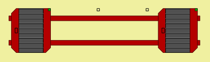
The rail transport system consists of a number of carts running on a rail. Each cart has a conveyor belt mounted on top to take and deliver workpieces. Currently, there is a fixed number of two carts, while the length of the rail is configurable.
For the below definition of signals and events, we use Z to indicate the cart, i.e., Z=1 for the west cart and Z=2 for the east cart. Furthermore, Y indicates positions on the rail, starting with Z=1 for the west-most position.
| signals | description | events |
|---|---|---|
| RS_BzM+, RS_BzM- | belt motor on cart z, to the south or north, resp. | rs_bZm+ (to the south), rs_bZm- (to the north), rs_bZoff (stop) |
| RS_BzWPS | workpiece sensor on cart z | rs_bZwpar (positive edge, arrival), rs_bZwplv (negative edge, departure) |
| RS_CzM+, DS_CzM- | drive cart z, to the east or west, resp. | rs_cZm+ (to the east), rs_cZm- (to the west), rs_cZoff (stop) |
| RS_PyS | cart is at position y | rs_pYcar (positive edge, arrival) rs_pYclv (negative edge, departure) |
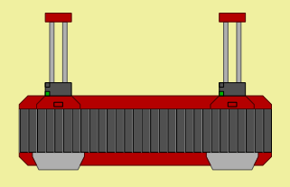
SF - Stack Feeder
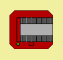
The stack feeder hosts a stack of workpieces which can be fed to the east. For this purpose, there are two pusher bars mounted on the feed belt, one of them visible as a vertical bar in the figure to the left. When the feed motor is on, the lowest workpiece of the stack is fed by the pusher. There is a sensor to indicate that a pusher is in the west-most position, aka home position. The mechanical setup is such that operating the feed motor until the other pusher arrives at the sensor will feed exactly one workpiece.
There is also a sensor to detect workpieces. After feeding a workpiece, the sensor will indicate the presence of the next workpiece until the stack is empty. The stack can be (re-)filled by user interaction (clicking the plus-symbol).
| signals | description | events |
|---|---|---|
| SF_FDM | feed motor | sf_fdon (feed motor on), sf_fdoff (feed motor off) |
| SF_FDS | pusher sensor | sf_fdhome (positive edge, pusher in home position), |
| SF_WPS | workpiece sensor | sf_wpar (positive edge, arrival), sf_wplv (negative edge, departure) |
XS - Exit Slide
Workpieces can exit the factory to the east via an exit slide. The slide can host up to four workpieces and must then be cleared by user interaction (click the forward/fast-forward symbol).
There is also a sensor to the west-most workpiece. Once the slide is occupied, there will be no negative edge on the respective sensor signal.
| signals | description | events |
|---|---|---|
| XS_WPS | workpiece sensor | xs_wpar (positive edge, arrival), xs_wplv (negative edge, departure) |
Advanced Topic: Faults
There is some support to simulate breakdown and repair of certain components, to be activated by their configuration menu; i.e., the context menu when simulation is halted. In the current implementation, considered faults affect the processing of workpieces by the universal processing machine and by the simple processing machine (fail to complete a process), as well as the sensor and motor of the conveyor belt (blind sensor and motor breakdown).
Each individual fault is considered either present or absent and, thus, can be thought of as a digital signal. A fault is referred to by a composed name XXXX_YYYY, where XXXX is the component name and YYYY indicates the particular fault; e.g., CB1_FM for a faulty belt motor FM of conveyor belt CB1. The configuration menu of relevant components allows to enable individual faults. Once enabled, the fault can be controlled manually by the Fault Monitor from the Simulation Menu. For CB1_FM, you can effectively disable the belt motor operation. In addition, each individual fault can be defined to occur periodically with parameter t_f the time until a failure occurs and with parameter t_r the time until the component recovers (parameter value 0 prevents periodic behaviour).
Each individual fault is associated with two external signals for explicit interaction with a supervisor (optional). The first signal has the suffix _D and exhibits sensor semantics to pass on the presence of the fault to the supervisor (fault detection). The second signal has the suffix _M and exhibits actuator semantics to allow the controller to reset the fault (maintenance). Each of the two signals has associated events for their respective edges; see the below table.
| signals | description | events |
|---|---|---|
| XXXX_YYYY_D | fault detection (sensor semantics) |
xxxx_yyyy_f (positive edge, occurence of the fault), xxxx_yyyy_r (negative edge, recovery complete) |
| XXXX_YYYY_M | maintenance control (actuator semantics) |
xxxx_yyyy_m (positive edge, apply maintenance), xxxx_yyyy_n (negative edge, normal operation) |
Note: External control, manual control, and periodic behaviour interfere in a non-trivial manner -- it is recommended to use one of the three mechanisms exclusively. The current implementation gives external maintenance the highest priority. As soon as XXXX_YYYY_M becomes active, any present fault is repaired instantly and no more faults will occur, neither manually nor periodically. When XXXX_YYYY_M becomes passive, timers get reset and the next periodic fault is re-scheduled. Manual control may now trigger and cure the fault before the timer elapses, either action resetting the respective timer.
Download/Installation/License
We have developed FlexFact to meet our requirements. However, due to limited resources, the current implementation misses some features one may expect. You are invited to download and inspect FlexFact, to see whether it is useful for your purposes.
A binary distribution of FlexFact is available from the LRT/FGDes download page, look for packages named faudes_applications_*. Supported operating systems:
Linux: The Linux package of FlexFact comes as .tar.gz archive. Extracting the archive, you obtain a folder faudes_applications, which you may place anywhere in the users file system. System-wide installation is currently not supported. To start FlexFact, run ~/faudes_flexfact/bin/flexfact from a command shell. The binaries are compiled for 64-bit Linux and link agains LSB stubs for cross-distribution compatibility. The most recent 32-bit binary is FlexFact 0.78, still available from the faudes archive. If you experience errors for missing libraries or unresolved symbols, please let us know. The DESTool installation details may be useful, too.
Mac OS: For Apple's Mac OS, FlexFact is distributed as a .dmg disk-image. Double click will mount the image and the finder will show the FlexFact application. It may be placed anywhere in the users file system. System-wide installation is currently not supported. The binary was built with the Mac OS 10.11 toolchain and should be compatible back to Mac OS 10.7, i.e., for Macs dated 2011 and thereafter. The most recent distribution that was actually compiled on Mac OS 10.7 is FlexFact 0.76, still available from the faudes archive
MS Windows: FlexFact is distributed as a setup.exe installer application. Double click will install by default to C:/Programs/FAUDES/Applications/FlexFact. Users need write permission on the installation folder in order for FlexFact to be operational. The MS Windows version of FlexFact was compiled for 64-bit MS Windows 7 and should be compatible with subsequent 64bit editions of MS Windows. You may need to install the MS Visual C redistributable package --- look for "vc_redist.x64.exe" for MS VS 2015. The most recent distribution compatible back to 32-bit MS Windows XP is FlexFact 0.78, available from the faudes archive.
Note: The application package is bundled with two other simulations, used for class-room experiments, namely ElePlant (a simple elevator) and SmallFact (a small factory). The bundle distribution simplifies our deployment mechanisms, please do not get confused by the further simulators.
Note: There is also a source package of FlexFact available from the LRT/FGDes download page. The sources are distributed under terms of the GPL. Please let us know, if you have different license requirements.